如果你也在 怎样代写电动力学Electrodynamics 这个学科遇到相关的难题，请随时右上角联系我们的24/7代写客服。电动力学Electrodynamics将光描述为频率范围约为1015赫兹的电磁辐射；在这个理论中，物质被视为连续的，主要的物质反应是电偏振。电动力学是关于变化的电场和磁场及其相互作用的理论，可广泛用于描述我们日常生活中遇到的许多现象。

电动力学Electrodynamics研究与运动中的带电体和变化的电场和磁场有关的现象（见电荷；电）；由于运动的电荷会产生磁场，所以电动力学关注磁、电磁辐射和电磁感应等效应，包括发电机和电动机等实际应用。电动力学的这一领域，通常被称为经典电动力学，是由物理学家詹姆斯-克拉克-麦克斯韦首次系统地解释的。麦克斯韦方程，一组微分方程，非常普遍地描述了这个领域的现象。最近的发展是量子电动力学，它的制定是为了解释电磁辐射与物质的相互作用，量子理论的规律适用于此。

avatest™帮您通过考试

avatest™的各个学科专家已帮了学生顺利通过达上千场考试。我们保证您快速准时完成各时长和类型的考试，包括in class、take home、online、proctor。写手整理各样的资源来或按照您学校的资料教您，创造模拟试题，提供所有的问题例子，以保证您在真实考试中取得的通过率是85%以上。如果您有即将到来的每周、季考、期中或期末考试，我们都能帮助您！

在不断发展的过程中，avatest™如今已经成长为论文代写，留学生作业代写服务行业的翘楚和国际领先的教育集团。全体成员以诚信为圆心，以专业为半径，以贴心的服务时刻陪伴着您， 用专业的力量帮助国外学子取得学业上的成功。

•最快12小时交付 

•200+ 英语母语导师 

•70分以下全额退款

物理代写|电动力学代考Electrodynamics代写|Electrostatics

Our intention is to move toward the general picture as quickly as possible, starting with a review of electrostatics. We take for granted the phenomenology of electric charge, including the Coulomb law of force between charges of dimensions that are small in comparison with their separation. This is expressed by the interaction energy, $E$, of a system of such charges in otherwise empty space, a vacuum:
$$
E=\frac{1}{2} \sum_{\substack{a, b \ a \neq b}} \frac{e_a e_b}{r_{a b}},
$$
where $e_a$ is the charge of the ath particle while
$$
r_{a b}=\left|\mathbf{r}_a-\mathbf{r}_b\right|
$$
is the separation between the ath and $b$ th particles. (Throughout this book we use the Gaussian system of units. Connection with the SI units will be given in Appendix A.) As we shall see, this starting point, the Coulomb energy (1.1), summarizes all the experimental facts of electrostatics. The energy of interaction of an individual charge with the rest of the system can be emphasized by rewriting (1.1) as
$$
E=\frac{1}{2} \sum_a e_a \sum_{b \neq a} \frac{e_b}{r_{a b}}=\frac{1}{2} \sum_a e_a \phi_a,
$$
where we have introduced the electrostatic potential at the location of the ath charge that is due to all the other charges,
$$
\phi_a=\sum_{b \neq a} \frac{e_b}{r_{a b}}
$$

物理代写|电动力学代考Electrodynamics代写|Inference of Maxwell’s Equations

We introduce time dependence in the simplest way by assuming that all charges are in uniform motion with a common velocity $\mathbf{v}$ as produced by transforming a static arrangement of charges to a coordinate system moving with velocity -v. (We insist that the same physics applies in the two situations.) At first we will take $|\mathbf{v}|$ to be very small in comparison with a critical speed $c$, which will be identified with the speed of light. To catch up with the moving charges, one would have to move with their velocity, $\mathbf{v}$. Accordingly, the time derivative in the co-moving coordinate system, in which the charges are at rest, is the sum of explicit time dependent and coordinate dependent contributions,
$$
\frac{d}{d t}=\frac{\partial}{\partial t}+\mathbf{v} \cdot \nabla
$$
so, in going from the static system to the uniformly moving system, we make the replacement
$$
\frac{\partial}{\partial t} \rightarrow \frac{d}{d t}=\frac{\partial}{\partial t}+\mathbf{v} \cdot \nabla
$$
The equation for the eonstancy of the charge density in (1.39) becomes, in the moving system
$$
0=\frac{\partial \rho}{\partial t} \rightarrow \frac{d \rho}{d t}=\frac{\partial \rho}{\partial t}+\mathbf{v} \cdot \nabla \rho
$$
or, since $\mathbf{v}$ is constant,
$$
\frac{\partial \rho}{\partial t}+\nabla \cdot(\mathbf{v} \rho)=0
$$
We recognize here a particular example of the charge flux vector or the (electric) current density $\mathbf{j}$,
$$
\mathbf{j}=\rho \mathbf{v}
$$

The relation between charge density and current density,
$$
\frac{\partial}{\partial t} \rho(\mathbf{r}, t)+\nabla \cdot \mathbf{j}(\mathbf{r}, t)=0
$$
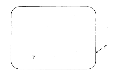
is the general statement of the conservation of charge. Conservation demands that the rate of decrease of the charge within an arbitrary volume $V$ must equal the rate at which the charge flows out of the bounding surface $S$, that is
$$
-\frac{d}{d t} \int_V(d \mathbf{r}) \rho(\mathbf{r}, t)=\oint_S d \mathbf{S} \cdot \mathbf{j}(\mathbf{r}, t)=\int_V(d \mathbf{r}) \boldsymbol{\nabla} \cdot \mathbf{j}(\mathbf{r}, t) .
$$
Since $V$ is arbitrary, the local conservation law, (1.45), follows. We also note that the expression for the current density, (1.44), continues to be valid even when $\mathbf{v}$ is dependent upon position, $\mathbf{v} \rightarrow \mathbf{v}(\mathbf{r}, t)$. (See Problem 1.4.)

We can perform a similar transformation on the equation for the electric field $\partial \mathbf{E} / \partial t=0$; namely,
$$
\mathbf{0}=\frac{d}{d t} \mathbf{E}=\frac{\partial \mathbf{E}}{\partial t}+(\mathbf{v} \cdot \boldsymbol{\nabla}) \mathbf{E} .
$$
Making use of a vector identity, together with (1.26) and (1.44), ( $\mathbf{v}$ is constant),
$$
\begin{aligned}
\boldsymbol{\nabla} \times(\mathbf{v} \times \mathbf{E}) & =\mathbf{v}(\boldsymbol{\nabla} \cdot \mathbf{E})-(\mathbf{v} \cdot \boldsymbol{\nabla}) \mathbf{E} \
& =\mathbf{v} 4 \pi \rho-(\mathbf{v} \cdot \boldsymbol{\nabla}) \mathbf{E} \
& =4 \pi \mathbf{j}-(\mathbf{v} \cdot \boldsymbol{\nabla}) \mathbf{E},
\end{aligned}
$$
we find an equation relating $\mathbf{E}$ to the current density,
$$
0=\frac{\partial \mathbf{E}}{\partial t}+4 \pi \mathbf{j}-\nabla \times(\mathbf{v} \times \mathbf{E})
$$

电动力学代写

物理代写|电动力学代考Electrodynamics代写|Electrostatics

我们的目的是从回顾静电学开始，尽快地走向总体情况。我们认为电荷的现象学是理所当然的，包括电荷之间的库仑力定律，这些电荷的尺寸与它们的分离相比是小的。这可以用这种电荷系统在真空中的相互作用能$E$来表示:
$$
E=\frac{1}{2} \sum_{\substack{a, b \ a \neq b}} \frac{e_a e_b}{r_{a b}},
$$
第4个粒子的电荷$e_a$在哪里
$$
r_{a b}=\left|\mathbf{r}a-\mathbf{r}_b\right| $$ 是ath和$b$粒子之间的距离。(在本书中，我们使用高斯单位制。与国际单位制单位的连接将在附录a中给出。我们将看到，库仑能(1.1)这个起点概括了静电学的所有实验事实。单个电荷与系统其余部分的相互作用能可以通过重写式(1.1)来强调 $$ E=\frac{1}{2} \sum_a e_a \sum{b \neq a} \frac{e_b}{r_{a b}}=\frac{1}{2} \sum_a e_a \phi_a,
$$
我们在最后一个电荷的位置引入了静电势这是由所有其他电荷引起的，
$$
\phi_a=\sum_{b \neq a} \frac{e_b}{r_{a b}}
$$

物理代写|电动力学代考Electrodynamics代写|Inference of Maxwell’s Equations

我们以最简单的方式引入时间依赖性，假设所有电荷以共同的速度$\mathbf{v}$匀速运动，这是通过将电荷的静态排列转换为以速度-v运动的坐标系而产生的。(我们坚持认为相同的物理原理适用于这两种情况。)首先，我们将$|\mathbf{v}|$与临界速度$c$相比非常小，这将与光速相一致。为了赶上移动的电荷，人们必须以它们的速度移动，$\mathbf{v}$。因此，在电荷处于静止状态的共动坐标系中，时间导数是与时间相关的显式贡献和与坐标相关的贡献的总和，
$$
\frac{d}{d t}=\frac{\partial}{\partial t}+\mathbf{v} \cdot \nabla
$$
所以，从静态系统到匀速运动系统，我们做了替换
$$
\frac{\partial}{\partial t} \rightarrow \frac{d}{d t}=\frac{\partial}{\partial t}+\mathbf{v} \cdot \nabla
$$
式(1.39)中电荷密度恒定的方程为，在运动系统中
$$
0=\frac{\partial \rho}{\partial t} \rightarrow \frac{d \rho}{d t}=\frac{\partial \rho}{\partial t}+\mathbf{v} \cdot \nabla \rho
$$
或者，因为$\mathbf{v}$是常数，
$$
\frac{\partial \rho}{\partial t}+\nabla \cdot(\mathbf{v} \rho)=0
$$
我们在这里认识到电荷通量矢量或(电)电流密度$\mathbf{j}$的一个特殊例子，
$$
\mathbf{j}=\rho \mathbf{v}
$$

电荷密度与电流密度的关系，
$$
\frac{\partial}{\partial t} \rho(\mathbf{r}, t)+\nabla \cdot \mathbf{j}(\mathbf{r}, t)=0
$$
是电荷守恒的一般表述。守恒定理要求任意体积内电荷的减少率$V$必须等于电荷流出边界面的速率$S$，即
$$
-\frac{d}{d t} \int_V(d \mathbf{r}) \rho(\mathbf{r}, t)=\oint_S d \mathbf{S} \cdot \mathbf{j}(\mathbf{r}, t)=\int_V(d \mathbf{r}) \boldsymbol{\nabla} \cdot \mathbf{j}(\mathbf{r}, t) .
$$
因为$V$是任意的，所以遵循本地守恒定律(1.45)。我们还注意到，即使$\mathbf{v}$依赖于位置$\mathbf{v} \rightarrow \mathbf{v}(\mathbf{r}, t)$，电流密度表达式(1.44)仍然有效。(见问题1.4)

我们可以对电场方程做一个类似的变换$\partial \mathbf{E} / \partial t=0$;即:
$$
\mathbf{0}=\frac{d}{d t} \mathbf{E}=\frac{\partial \mathbf{E}}{\partial t}+(\mathbf{v} \cdot \boldsymbol{\nabla}) \mathbf{E} .
$$
利用向量恒等式，加上(1.26)和式(1.44)，($\mathbf{v}$为常数)，
$$
\begin{aligned}
\boldsymbol{\nabla} \times(\mathbf{v} \times \mathbf{E}) & =\mathbf{v}(\boldsymbol{\nabla} \cdot \mathbf{E})-(\mathbf{v} \cdot \boldsymbol{\nabla}) \mathbf{E} \
& =\mathbf{v} 4 \pi \rho-(\mathbf{v} \cdot \boldsymbol{\nabla}) \mathbf{E} \
& =4 \pi \mathbf{j}-(\mathbf{v} \cdot \boldsymbol{\nabla}) \mathbf{E},
\end{aligned}
$$
我们找到了$\mathbf{E}$与电流密度有关的方程，
$$
0=\frac{\partial \mathbf{E}}{\partial t}+4 \pi \mathbf{j}-\nabla \times(\mathbf{v} \times \mathbf{E})
$$

物理代写|电动力学代考Electrodynamics代写 请认准exambang™. exambang™为您的留学生涯保驾护航。

在当今世界，学生正面临着越来越多的期待，他们需要在学术上表现优异，所以压力巨大。

avatest.org 为您提供可靠及专业的论文代写服务以便帮助您完成您学术上的需求，让您重新掌握您的人生。我们将尽力给您提供完美的论文，并且保证质量以及准时交稿。除了承诺的奉献精神，我们的专业写手、研究人员和校对员都经过非常严格的招聘流程。所有写手都必须证明自己的分析和沟通能力以及英文水平，并通过由我们的资深研究人员和校对员组织的面试。

其中代写论文大多数都能达到A，B 的成绩， 从而实现了零失败的目标。

这足以证明我们的实力。选择我们绝对不会让您后悔，选择我们是您最明智的选择！

微观经济学代写

微观经济学是主流经济学的一个分支，研究个人和企业在做出有关稀缺资源分配的决策时的行为以及这些个人和企业之间的相互作用。my-assignmentexpert™ 为您的留学生涯保驾护航 在数学Mathematics作业代写方面已经树立了自己的口碑, 保证靠谱, 高质且原创的数学Mathematics代写服务。我们的专家在图论代写Graph Theory代写方面经验极为丰富，各种图论代写Graph Theory相关的作业也就用不着 说。

线性代数代写

线性代数是数学的一个分支，涉及线性方程，如：线性图，如：以及它们在向量空间和通过矩阵的表示。线性代数是几乎所有数学领域的核心。

博弈论代写

现代博弈论始于约翰-冯-诺伊曼（John von Neumann）提出的两人零和博弈中的混合策略均衡的观点及其证明。冯-诺依曼的原始证明使用了关于连续映射到紧凑凸集的布劳威尔定点定理，这成为博弈论和数学经济学的标准方法。在他的论文之后，1944年，他与奥斯卡-莫根斯特恩（Oskar Morgenstern）共同撰写了《游戏和经济行为理论》一书，该书考虑了几个参与者的合作游戏。这本书的第二版提供了预期效用的公理理论，使数理统计学家和经济学家能够处理不确定性下的决策。

微积分代写

微积分，最初被称为无穷小微积分或 “无穷小的微积分”，是对连续变化的数学研究，就像几何学是对形状的研究，而代数是对算术运算的概括研究一样。

它有两个主要分支，微分和积分；微分涉及瞬时变化率和曲线的斜率，而积分涉及数量的累积，以及曲线下或曲线之间的面积。这两个分支通过微积分的基本定理相互联系，它们利用了无限序列和无限级数收敛到一个明确定义的极限的基本概念 。

计量经济学代写

什么是计量经济学？
计量经济学是统计学和数学模型的定量应用，使用数据来发展理论或测试经济学中的现有假设，并根据历史数据预测未来趋势。它对现实世界的数据进行统计试验，然后将结果与被测试的理论进行比较和对比。

根据你是对测试现有理论感兴趣，还是对利用现有数据在这些观察的基础上提出新的假设感兴趣，计量经济学可以细分为两大类：理论和应用。那些经常从事这种实践的人通常被称为计量经济学家。

MATLAB代写

MATLAB 是一种用于技术计算的高性能语言。它将计算、可视化和编程集成在一个易于使用的环境中，其中问题和解决方案以熟悉的数学符号表示。典型用途包括：数学和计算算法开发建模、仿真和原型制作数据分析、探索和可视化科学和工程图形应用程序开发，包括图形用户界面构建MATLAB 是一个交互式系统，其基本数据元素是一个不需要维度的数组。这使您可以解决许多技术计算问题，尤其是那些具有矩阵和向量公式的问题，而只需用 C 或 Fortran 等标量非交互式语言编写程序所需的时间的一小部分。MATLAB 名称代表矩阵实验室。MATLAB 最初的编写目的是提供对由 LINPACK 和 EISPACK 项目开发的矩阵软件的轻松访问，这两个项目共同代表了矩阵计算软件的最新技术。MATLAB 经过多年的发展，得到了许多用户的投入。在大学环境中，它是数学、工程和科学入门和高级课程的标准教学工具。在工业领域，MATLAB 是高效研究、开发和分析的首选工具。MATLAB 具有一系列称为工具箱的特定于应用程序的解决方案。对于大多数 MATLAB 用户来说非常重要，工具箱允许您学习和应用专业技术。工具箱是 MATLAB 函数（M 文件）的综合集合，可扩展 MATLAB 环境以解决特定类别的问题。可用工具箱的领域包括信号处理、控制系统、神经网络、模糊逻辑、小波、仿真等。