如果你也在 怎样代写电动力学Electrodynamics 这个学科遇到相关的难题，请随时右上角联系我们的24/7代写客服。电动力学Electrodynamics将光描述为频率范围约为1015赫兹的电磁辐射；在这个理论中，物质被视为连续的，主要的物质反应是电偏振。电动力学是关于变化的电场和磁场及其相互作用的理论，可广泛用于描述我们日常生活中遇到的许多现象。

电动力学Electrodynamics研究与运动中的带电体和变化的电场和磁场有关的现象（见电荷；电）；由于运动的电荷会产生磁场，所以电动力学关注磁、电磁辐射和电磁感应等效应，包括发电机和电动机等实际应用。电动力学的这一领域，通常被称为经典电动力学，是由物理学家詹姆斯-克拉克-麦克斯韦首次系统地解释的。麦克斯韦方程，一组微分方程，非常普遍地描述了这个领域的现象。最近的发展是量子电动力学，它的制定是为了解释电磁辐射与物质的相互作用，量子理论的规律适用于此。

avatest™帮您通过考试

avatest™的各个学科专家已帮了学生顺利通过达上千场考试。我们保证您快速准时完成各时长和类型的考试，包括in class、take home、online、proctor。写手整理各样的资源来或按照您学校的资料教您，创造模拟试题，提供所有的问题例子，以保证您在真实考试中取得的通过率是85%以上。如果您有即将到来的每周、季考、期中或期末考试，我们都能帮助您！

在不断发展的过程中，avatest™如今已经成长为论文代写，留学生作业代写服务行业的翘楚和国际领先的教育集团。全体成员以诚信为圆心，以专业为半径，以贴心的服务时刻陪伴着您， 用专业的力量帮助国外学子取得学业上的成功。

•最快12小时交付 

•200+ 英语母语导师 

•70分以下全额退款

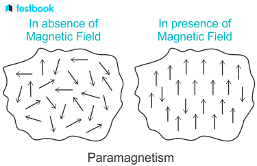
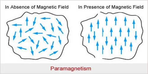
物理代写|电动力学代考Electrodynamics代写|Paramagnetism

What happens if there is a permanent intrinsic moment,
$$
\boldsymbol{\mu}_0 \neq \mathbf{0} \text { ? }
$$

This situation is analogous to that of permanent electric dipole moments, discussed in Section 5.4. Due to thermal motion, the average magnetization will be zero if there is no external field. In the presence of a magnetic field, we obtain the thermal averaged magnetic moment from (5.64) by replacing $d$ by $\mu_0$ and E by $\mathbf{B}$. The obvious high temperature limit, from (5.68), is
$$
\left\langle\boldsymbol{\mu}0\right\rangle_T=\frac{\mu_0^2}{3 k T} \mathbf{B} $$ corresponding to the magnetization $$ \mathbf{M}=\frac{n \mu_0^2}{3 k T} \mathbf{B} . $$ This is appropriate to the weak field circumstance $$ \mu_0 B \ll k T \text {. } $$ Inasmuch as the typical magnitudes of $\mu_0 / d$ are of order $v / c \sim 10^{-2}-10^{-3}$, the upper limit to $B$, at room temperature, for $(6.42)$ to be valid is in the range of millions of gauss, or hundreds of Teslas. Note that unlike in diamagnetism, the magnetization here is parallel to the magnetic field. The permeability is [cf. $(6.38)$ ] $$ \mu=\frac{1}{1-4 \pi n \frac{\mu_0^2}{3 k T}} \approx 1+4 \pi n \frac{\mu_0^2}{3 k T}>1, \quad \chi_m=n \frac{\mu_0^2}{3 k T}, $$ since, again, the magnetization is small. Substances with positive magnetic susceptibilities are called paramagnetic. For this class of materials, the permeability is greater than one. The simple models indicate that the ratio of paramagnetic to diamagnetic susceptibilities is of the order $$ \frac{\chi{m, \text { para }}}{\chi_{m, \text { dia }}} \sim \frac{m v^2}{k T} \sim 100 \text { at room temperature, }
$$
where $m v^2$ is related to the magnitude of energies in the atom. The estimate in (6.45) is in general agreement with the observation that paramagnetic gaseous oxygen at standard pressure and room temperature has a positive susceptibility about one fifth the susceptibility of water, although the molecular density of the oxygen is less than a thousandth of that of water. The susceptibilities of paramagnetic substances are still so small compared with unity (for liquid oxygen, $\chi_m=3 \times 10^{-4}$ ) that the approximation of neglecting the distinction between $\mathbf{B}$ and $\mathbf{H}$ in (6.44) is well justified. The inverse dependence on temperature displayed there was discovered experimentally by Pierre Curie (1859-1906).

物理代写|电动力学代考Electrodynamics代写|Ferromagnetism

The history of magnetism did not begin with the phenomena of paramagnetism and diamagnetism, which were first recognized by Faraday in 1845 . The ancients were familiar with the remarkable properties of Magnesian stone, the iron oxide $\mathrm{Fe}3 \mathrm{O}_4$. The term ferromagnetism refers to the property of such substances, primarily members of the iron group, of exhibiting permanent magnetization. A simple model of this effect was introduced by Pierre Weiss (1865-1940), who effectively postulated that the driving magnetic field within ferromagnets is not $(6.50)$, but rather $$ \mathbf{B}{\text {driving }}=\mathbf{H}+\lambda \mathbf{M} \text {, }
$$
where $\lambda \gg 1$. In terms of $\mathbf{B}_{\text {driving }}$ we wish to calculate the thermal average of the intrinsic magnetic moment, $\left\langle\boldsymbol{\mu}_0\right\rangle_T$. Rather than use a classical distribution (but see Problem 6.3), it is simpler and more accurate quantum mechanically to suppose that the atomic magnetic moment $\boldsymbol{\mu}0$ is either lined up parallel or anti-parallel to $\mathbf{B}{\text {driving }}$, which defines the $z$ axis. Since the interaction energies, for the two possibilities, are
$$
-\mu_0 \cdot \mathbf{B}{\text {driving }}=\mp \mu_0 B{\text {driving }},
$$
the Boltzmann weighting of states yields
$$
\left\langle\mu_{0 z}\right\rangle_T=\frac{\mu_0 e^x-\mu_0 e^{-x}}{e^x+e^{-x}}=\mu_0 \tanh x,
$$
with
$$
x=\frac{\mu_0}{k T}(H+\lambda M) .
$$
The resulting magnetization has magnitude
$$
M=n \mu_0 \tanh \frac{\mu_0}{k T}(H+\lambda M) .
$$
The possible existence of a magnetization in the absence of the field $H$ is implied by the equation
$$
\frac{M}{n \mu_0}=\tanh \left(\frac{T_c}{T} \frac{M}{n \mu_0}\right)
$$
in which
$$
T_c \equiv \frac{n \mu_0^2}{k} \lambda
$$

电动力学代写

物理代写|电动力学代考Electrodynamics代写|Paramagnetism

如果有一个永久的内在时刻，
$$
\boldsymbol{\mu}_0 \neq \mathbf{0} \text { ? }
$$

这种情况类似于5.4节讨论的永久电偶极矩。由于热运动，如果没有外场，平均磁化强度将为零。在磁场存在的情况下，我们通过将$d$替换为$\mu_0$，将E替换为$\mathbf{B}$，得到式(5.64)中的热平均磁矩。从(5.68)开始，明显的高温极限为
$$
\left\langle\boldsymbol{\mu}0\right\rangle_T=\frac{\mu_0^2}{3 k T} \mathbf{B} $$对应磁化强度$$ \mathbf{M}=\frac{n \mu_0^2}{3 k T} \mathbf{B} . $$这适用于弱场情况$$ \mu_0 B \ll k T \text {. } $$由于$\mu_0 / d$的典型数量级为$v / c \sim 10^{-2}-10^{-3}$，在室温下，$(6.42)$有效的上限为$B$，在数百万高斯或数百特斯拉的范围内。注意，不像抗磁性，这里的磁化平行于磁场。磁导率为[cf. $(6.38)$] $$ \mu=\frac{1}{1-4 \pi n \frac{\mu_0^2}{3 k T}} \approx 1+4 \pi n \frac{\mu_0^2}{3 k T}>1, \quad \chi_m=n \frac{\mu_0^2}{3 k T}, $$，因为磁化强度也很小。具有正磁化率的物质称为顺磁性的。对于这类材料，磁导率大于1。简单模型表明，顺磁磁化率与抗磁磁化率之比约为$$ \frac{\chi{m, \text { para }}}{\chi_{m, \text { dia }}} \sim \frac{m v^2}{k T} \sim 100 \text { at room temperature, }
$$
其中$m v^2$与原子能量的大小有关。(6.45)中的估计与下述观察大体一致:在标准压力和室温下，顺磁性气态氧的磁化率约为水的五分之一，尽管氧的分子密度小于水的千分之一。顺磁性物质的磁化率与统一相比仍然很小(对于液氧，$\chi_m=3 \times 10^{-4}$)，因此在(6.44)中忽略$\mathbf{B}$和$\mathbf{H}$之间的区别的近似是很合理的。皮埃尔·居里(Pierre Curie, 1859-1906)在实验中发现了与温度相反的依赖性。

物理代写|电动力学代考Electrodynamics代写|Ferromagnetism

磁学的历史并不是从顺磁性和抗磁性现象开始的，这两种现象是法拉第在1845年首先发现的。古人很熟悉镁石中氧化铁的显著特性$\mathrm{Fe}3 \mathrm{O}4$。铁磁性一词是指这些主要是铁族成员的物质具有永久磁化的性质。皮埃尔·韦斯(Pierre Weiss, 1865-1940)提出了一个简单的模型，他有效地假设了铁磁体内部的驱动磁场不是$(6.50)$，而是$$ \mathbf{B}{\text {driving }}=\mathbf{H}+\lambda \mathbf{M} \text {, } $$ 在哪里$\lambda \gg 1$。根据$\mathbf{B}{\text {driving }}$，我们希望计算本征磁矩$\left\langle\boldsymbol{\mu}0\right\rangle_T$的热平均值。与其使用经典分布(参见问题6.3)，不如从量子力学角度假设原子磁矩$\boldsymbol{\mu}0$与$\mathbf{B}{\text {driving }}$平行或反平行，从而定义$z$轴，这更简单、更准确。因为这两种可能性的相互作用能是 $$ -\mu_0 \cdot \mathbf{B}{\text {driving }}=\mp \mu_0 B{\text {driving }}, $$ 状态的玻尔兹曼加权 $$ \left\langle\mu{0 z}\right\rangle_T=\frac{\mu_0 e^x-\mu_0 e^{-x}}{e^x+e^{-x}}=\mu_0 \tanh x,
$$
有
$$
x=\frac{\mu_0}{k T}(H+\lambda M) .
$$
产生的磁化强度是有大小的
$$
M=n \mu_0 \tanh \frac{\mu_0}{k T}(H+\lambda M) .
$$
在没有场$H$的情况下，磁化的可能存在是由方程暗示的
$$
\frac{M}{n \mu_0}=\tanh \left(\frac{T_c}{T} \frac{M}{n \mu_0}\right)
$$
其中
$$
T_c \equiv \frac{n \mu_0^2}{k} \lambda
$$

物理代写|电动力学代考Electrodynamics代写 请认准exambang™. exambang™为您的留学生涯保驾护航。

在当今世界，学生正面临着越来越多的期待，他们需要在学术上表现优异，所以压力巨大。

avatest.org 为您提供可靠及专业的论文代写服务以便帮助您完成您学术上的需求，让您重新掌握您的人生。我们将尽力给您提供完美的论文，并且保证质量以及准时交稿。除了承诺的奉献精神，我们的专业写手、研究人员和校对员都经过非常严格的招聘流程。所有写手都必须证明自己的分析和沟通能力以及英文水平，并通过由我们的资深研究人员和校对员组织的面试。

其中代写论文大多数都能达到A，B 的成绩， 从而实现了零失败的目标。

这足以证明我们的实力。选择我们绝对不会让您后悔，选择我们是您最明智的选择！

微观经济学代写

微观经济学是主流经济学的一个分支，研究个人和企业在做出有关稀缺资源分配的决策时的行为以及这些个人和企业之间的相互作用。my-assignmentexpert™ 为您的留学生涯保驾护航 在数学Mathematics作业代写方面已经树立了自己的口碑, 保证靠谱, 高质且原创的数学Mathematics代写服务。我们的专家在图论代写Graph Theory代写方面经验极为丰富，各种图论代写Graph Theory相关的作业也就用不着 说。

线性代数代写

线性代数是数学的一个分支，涉及线性方程，如：线性图，如：以及它们在向量空间和通过矩阵的表示。线性代数是几乎所有数学领域的核心。

博弈论代写

现代博弈论始于约翰-冯-诺伊曼（John von Neumann）提出的两人零和博弈中的混合策略均衡的观点及其证明。冯-诺依曼的原始证明使用了关于连续映射到紧凑凸集的布劳威尔定点定理，这成为博弈论和数学经济学的标准方法。在他的论文之后，1944年，他与奥斯卡-莫根斯特恩（Oskar Morgenstern）共同撰写了《游戏和经济行为理论》一书，该书考虑了几个参与者的合作游戏。这本书的第二版提供了预期效用的公理理论，使数理统计学家和经济学家能够处理不确定性下的决策。

微积分代写

微积分，最初被称为无穷小微积分或 “无穷小的微积分”，是对连续变化的数学研究，就像几何学是对形状的研究，而代数是对算术运算的概括研究一样。

它有两个主要分支，微分和积分；微分涉及瞬时变化率和曲线的斜率，而积分涉及数量的累积，以及曲线下或曲线之间的面积。这两个分支通过微积分的基本定理相互联系，它们利用了无限序列和无限级数收敛到一个明确定义的极限的基本概念 。

计量经济学代写

什么是计量经济学？
计量经济学是统计学和数学模型的定量应用，使用数据来发展理论或测试经济学中的现有假设，并根据历史数据预测未来趋势。它对现实世界的数据进行统计试验，然后将结果与被测试的理论进行比较和对比。

根据你是对测试现有理论感兴趣，还是对利用现有数据在这些观察的基础上提出新的假设感兴趣，计量经济学可以细分为两大类：理论和应用。那些经常从事这种实践的人通常被称为计量经济学家。

MATLAB代写

MATLAB 是一种用于技术计算的高性能语言。它将计算、可视化和编程集成在一个易于使用的环境中，其中问题和解决方案以熟悉的数学符号表示。典型用途包括：数学和计算算法开发建模、仿真和原型制作数据分析、探索和可视化科学和工程图形应用程序开发，包括图形用户界面构建MATLAB 是一个交互式系统，其基本数据元素是一个不需要维度的数组。这使您可以解决许多技术计算问题，尤其是那些具有矩阵和向量公式的问题，而只需用 C 或 Fortran 等标量非交互式语言编写程序所需的时间的一小部分。MATLAB 名称代表矩阵实验室。MATLAB 最初的编写目的是提供对由 LINPACK 和 EISPACK 项目开发的矩阵软件的轻松访问，这两个项目共同代表了矩阵计算软件的最新技术。MATLAB 经过多年的发展，得到了许多用户的投入。在大学环境中，它是数学、工程和科学入门和高级课程的标准教学工具。在工业领域，MATLAB 是高效研究、开发和分析的首选工具。MATLAB 具有一系列称为工具箱的特定于应用程序的解决方案。对于大多数 MATLAB 用户来说非常重要，工具箱允许您学习和应用专业技术。工具箱是 MATLAB 函数（M 文件）的综合集合，可扩展 MATLAB 环境以解决特定类别的问题。可用工具箱的领域包括信号处理、控制系统、神经网络、模糊逻辑、小波、仿真等。